Risk is not one number: volatility, VaR, conditional VaR and drawdown measure different things

A USD 10,000 portfolio with 4% monthly volatility sounds under control. But that figure does not say how much can be lost in a bad month, how severe the worst scenario is when the calculation fails, or how long the portfolio can sit below its peak. Each of those questions needs a different measure.

The most common mistake in measuring risk is keeping one number and treating it as if it explained everything. A single number summarizes one dimension of risk and leaves the others unmeasured.

The risk of a portfolio is not one number but a set of measures, and each exists because the others leave something unanswered.

Volatility: how much it moves

It is measured as the standard deviation of returns. If returns approximate a normal distribution, about 68% of periods fall within one standard deviation of the average, about 95% within two and about 99.7% within three.

With 4% monthly volatility, a typical month moves up to 4% in each direction, or USD 400 on USD 10,000. It is the starting point of almost every financial model. Its limit is that it treats rises and falls the same and says little about extremes.

Value at risk: where the problem begins

Value at risk (VaR) answers a specific question: at a given confidence level, what is the loss that should not be exceeded over a period? In its simplest parametric version, with a zero mean, it is volatility multiplied by a factor from the normal distribution: 1.645 for 95% and 2.326 for 99%.

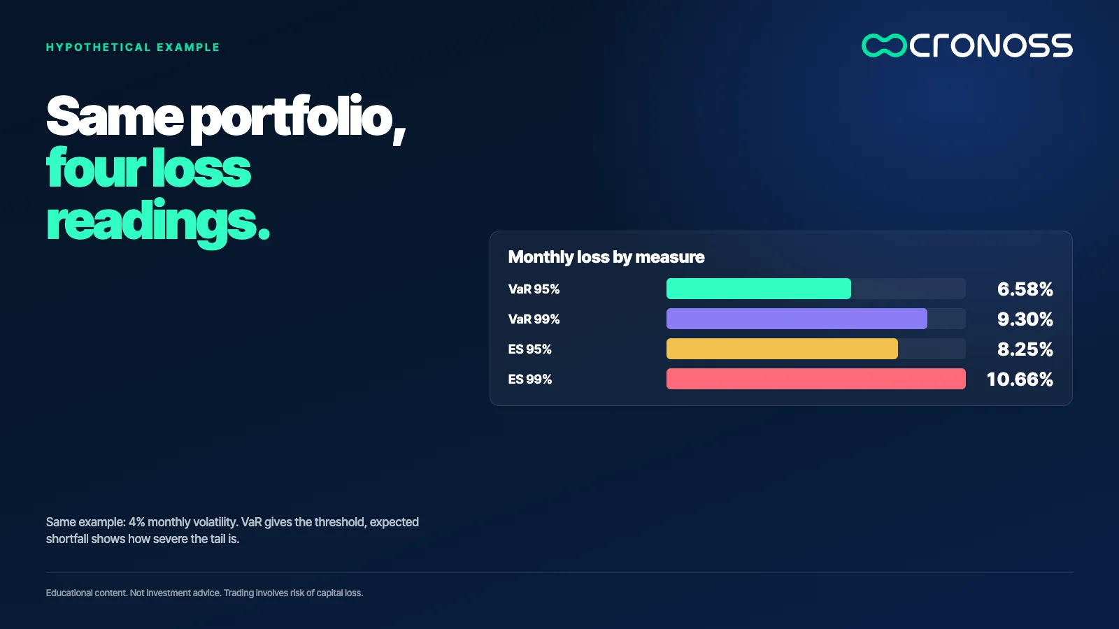
With the same example: 4% x 1.645 = 6.58%, which is a USD 658 maximum loss at 95% confidence; at 99%, 9.30% or USD 930. The correct reading is probabilistic: in 5% of months the loss can be larger than USD 658, and VaR does not say by how much.

Conditional loss: how bad it gets after that

That omission is what conditional VaR, or expected shortfall, corrects: the average of the losses in the cases where VaR was already exceeded. For a normal distribution and 4% volatility, it is about 8.25% at 95% confidence (USD 825) and 10.66% at 99% (USD 1,066).

The gap between VaR and this measure indicates how severe the tail is. When tails are heavier than a normal distribution's, as in real crises, the gap is larger, which is why this measure is used alongside VaR and not in its place.

Drawdown: what it feels like, not just what it computes

The earlier measures are statistics over a period. Drawdown measures the experience of traveling the path: the fall from the previous peak to the later trough. If a portfolio rises from USD 10,000 to USD 12,000 and then drops to USD 9,000, the drawdown is (9,000 - 12,000) / 12,000 = -25%.

An asset can have moderate volatility and still accumulate deep drops, because drawdown adds up consecutive negative moves. It is the measure closest to what the person investing actually lives through.

Volatility is not constant

Calculating a fixed standard deviation assumes the market behaves the same all the time. In practice there are calm periods and turbulent ones. Adaptive models, such as the exponentially weighted moving average (EWMA) and the GARCH family, give more weight to recent data so the estimate reacts when conditions change.

The underlying idea is that volatility is a process that gets updated, not a number calculated once. A VaR computed with last year's volatility can fall short in a turbulent month.

How much noise sits inside the move

There is another dimension: not only how much the price moves, but how direct the path is. The efficiency ratio compares the net change between two points with the total distance the price traveled. If it goes from 100 to 104 over five periods with back-and-forth moves of 3, 2, 4, 3 and 2 points, the path adds up to 14 and the efficiency is 4 / 14 = 0.29. If it reaches 104 in four clean steps of 1 point, the efficiency is 1.

Noise is 1 minus efficiency. Two assets with the same volatility can have very different noise levels, and that difference matters when deciding how much confidence to place in a signal.

A clean backtest is the beginning, not the proof

Risk measures are also used to evaluate an investment rule before using it. A backtest runs through historical data and calculates how it would have gone, but its first version is usually an optimistic one. There are four precautions:

• Separate the edge from the costs, without forgetting them. It is valid to start without commissions or price spreads to detect whether any edge exists. But the resulting curve looks smooth precisely because costs are missing. With an average gross gain of USD 6 per trade and a cost of USD 5, what remains is USD 1, and the more trades there are, the more the costs weigh.
• More trades give more significance, not more truth. A rule that produces 41 trades on a daily timeframe gives little data. The same pattern with 236 trades, when moved to a shorter timeframe, cuts the standard error of the mean by a factor of square root(236 / 41), about 2.4. It allows testing and filtering, but each adjustment made on the same data pushes the rule closer to overfitting.
• Numbers that are too perfect are a warning sign. A record with not a single loss or no drawdown is not realistic: every rule has trades that hit the loss limit, and tightening that limit makes it happen more often. Words like "never" and "always" do not belong in a statistic.
• Drawdown outranks return. A rule can show an attractive curve and still have drawdowns nobody would sustain. Placing a loss limit reduces them, but sometimes it damages the curve; that balance is measured, not assumed.

A mediocre but stable result usually means there is something to polish, not that the idea is ready. From there to a real account there are intermediate stages: checking whether the pattern is overfit, whether it exploits a real edge, and whether it degrades when parameters change. It is almost a discipline of its own.

What to check when measuring a portfolio or a rule

1. Calculate volatility, VaR and conditional VaR for the same portfolio and compare them. If the gap between the last two is large, the tail is heavy.
2. Calculate the historical maximum drawdown and ask yourself whether you could stick to the plan through that fall.
3. Test the model on data you did not use to build it, with costs included, and check how much the result changes if you nudge the parameters. Past results do not guarantee future results.

Measuring is not predicting

None of these measures removes risk or anticipates what comes next. What they offer is an orderly way to stop saying "this portfolio is risky" and start saying "this portfolio has this volatility, this tail loss and this historical drawdown". A risk that can be described with numbers can be compared, limited and reviewed.

If you want to calculate these measures step by step and use them to optimize a portfolio with models such as Markowitz, minimum variance and risk parity, the program Medición y Optimización de Portafolios (Portfolio Measurement and Optimization) covers the full path: see the program.

Educational content. Cronoss is not a broker, investment firm or financial adviser, and nothing above is an investment recommendation.