Key takeaways
- Correlation between assets measures how consistently two prices move in the same direction.
- In trading it is calculated with the Pearson coefficient, a number between −1 and +1.
- The coefficient measures directional synchrony, not the size of the move.
- In the lead-lag effect, one asset anticipates another, and the gap only has meaning while the correlation stays firm.
- Correlation changes with every candle: measure it at the moment of deciding and with a window adjusted to the timeframe.
Two indices can show a correlation of 0.90 and still move out of sync.
Correlation between assets measures how consistently two prices move in the same direction. In trading, it is calculated with the Pearson coefficient, a number between −1 and +1 that summarizes that relationship. A value close to +1 indicates that the two assets rise and fall together. A value close to −1 indicates that they move as mirror images.
For short-term traders, correlation matters most in the moments when it breaks down. That gap between an asset and its pair holds the useful information. This article explains how correlation is measured, why lag appears and how to check for yourself whether it exists.
What does the Pearson coefficient measure?
The Pearson coefficient measures the strength of the linear relationship between two price series. It answers a specific question: when one asset moves, how consistently does the other move in the same direction?
The calculation compares the moves of both assets period by period. If one asset's rises almost always coincide with the other's rises, the result approaches +1. If one asset's rises coincide with the other's falls, it approaches −1. Without a pattern, the value hovers around zero.
The coefficient measures directional synchrony and leaves out the size of the move. Two assets can show a correlation of 0.95 even if one rises twice as much as the other on every candle. This detail matters later, when you need to project how far the lagging asset can go.
The Cronoss class on this topic uses Nasdaq and S&P 500 futures as its reference pair. For scalping, which means trading moves of seconds or a few minutes, instructor Yecid Fuentes only considers pairs with a coefficient above 0.85 or 0.90. Below 0.80, he treats the link as broken.
Why does one asset move before its pair?
One asset moves ahead of its pair because the two markets do not process the same information at the same pace. Even when they share drivers, each asset has its own participants, its own liquidity and its own pending orders. One reacts first. The other takes its time.
That gap is called the lead-lag effect, the pattern in which one asset anticipates another. The leader sets the direction. The laggard follows it with a delay of a few seconds or minutes.
The class explains it with an elastic leash. A person walks their dog on a stretchy leash. When the person starts moving, the dog takes a moment to react, but the tension in the leash pulls it in the same direction.
In that image, the correlation coefficient measures how taut the leash is. While the leash holds, the gap the leader opens tends to close. If the leash breaks, each one goes its own way and the gap stops meaning anything.
The logic also works with negative correlation. The class includes cases where the indicator line sticks to −1. There, the gap is read in reverse, and a rise in the leader anticipates a fall in the laggard.
The lag only has meaning while the coefficient confirms that the link is still firm. That condition orders everything else.
What lookback window should you use to measure correlation?
The calculation window should match the timeframe you trade. The coefficient is calculated over a fixed number of past candles, and that number determines how quickly it reflects changes in the relationship.
A 50-period window on a one-minute chart describes the average relationship over almost an hour. For a decision that is made and resolved in a few minutes, that average arrives too late. A short window captures the relationship of the moment, at the cost of more noise in the reading.
The class proposes a short window for one- to five-minute charts. The platform's default value rarely matches the timeframe of a scalper.
No factory setting works for every timeframe. Anyone measuring correlation should choose the window before reading the number.
What does the lead-lag effect look like in numbers?
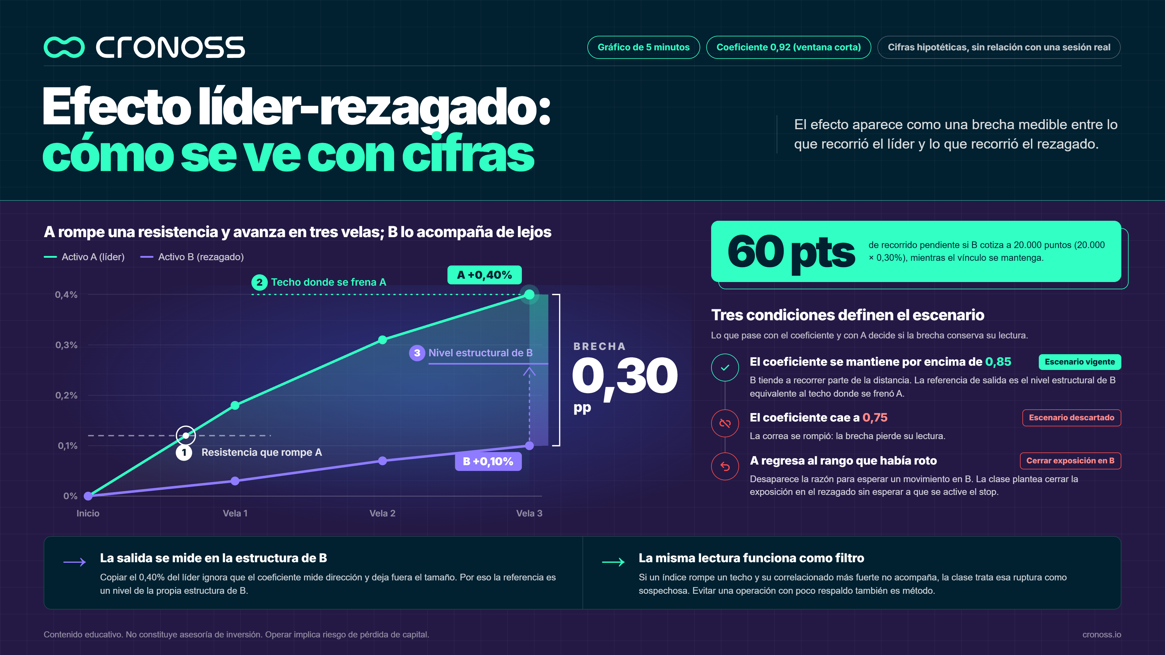
The effect shows up as a measurable gap between how far the leader moved and how far the laggard moved. The figures that follow are hypothetical and do not correspond to a real session.
Two assets, A and B, show a coefficient of 0.92 on the short window of a 5-minute chart. A breaks a resistance and rises 0.40% in three candles. B, over the same period, rises 0.10%.
The gap is 0.30 percentage points. If B trades at 20,000 points, that gap equals 60 points of pending movement as long as the link holds.
From there, the scenario depends on three conditions:
- The coefficient stays above 0.85. The class reads this as B tending to cover part of the distance. The exit reference is B's structural level equivalent to the ceiling where A stalled.
- The coefficient falls to 0.75. The leash has broken, the gap loses its meaning and the scenario is discarded.
- A returns to the range it had broken. The reason to expect a move in B disappears. The class suggests closing the exposure in the laggard without waiting for the stop to trigger.
The exit reference uses a level from B's structure. Copying A's 0.40% move ignores that the coefficient measures direction and leaves out size.
The same reading works as a filter. If an index breaks a ceiling and its strongest correlated asset does not follow, the class treats that breakout as suspicious. Avoiding a trade with little support is also part of the method.
What mistakes do people make when using correlations?
The two most common mistakes are treating correlation as a fixed data point and reading the lag as a promise.
Treating correlation as a fixed data point
The coefficient describes the relationship over the latest candles and changes with every new candle. A trader who checks a pair's correlation once and treats it as valid for the whole session is trading on an expired data point.
The relationship between two assets reflects what is moving each of them at that moment. When a data release or news affects one market more than the other, their moves separate and the coefficient falls within a few candles.
The leash can break at any time. That is why the class's criterion requires checking the coefficient at the moment of the decision, with the indicator line pinned at +1 or −1.
Reading the lag as a promise
The lag describes a probability and depends on the leader sustaining its move. If the leader makes a false breakout and returns to its range, the laggard loses its reason to move.
The mistake has a variant: expecting the laggard to cover the same percentage as the leader. The coefficient never promised magnitude. A calmer asset can follow the direction with half the move.
How do you test the effect on your own chart?
The test consists of reviewing the history of two correlated assets and counting how many gaps closed. Anyone can do it with their platform's history, without opening trades:
- Open two 5-minute charts of assets that tend to move together.
- Insert the correlation coefficient indicator with a short window.
- Look through the history for moments when one rose sharply and the other did not.
- Note the coefficient's value at that moment and whether the gap closed in the following candles.
The result is falsifiable. If gaps closed more often when the coefficient was above 0.85 than when it was below 0.80, the criterion has support for that pair. If no difference appears, the criterion does not hold for that pair and that timeframe.
A sample of ten or twenty cases is already enough to see whether the pattern repeats or was an isolated coincidence.
What does correlation add to a technical decision?
Correlation turns an isolated chart into a reading of two connected markets. Its usefulness depends on a specific discipline: measuring the coefficient in the right window, at the moment of deciding, and accepting that the leader can also fail.
Those who use it this way gain a second source of confirmation and a clear rule for discarding scenarios. Those who use it as an automatic signal inherit the leader's mistakes without knowing it.
Yecid Fuentes develops this logic in the class Scalping y Correlaciones Líder-Rezagado (Scalping and Lead-Lag Correlations), Module 3 of the program Análisis Técnico Avanzado de Mercados Financieros (Advanced Technical Analysis of Financial Markets). That module connects correlation with volatility: another of its classes uses ATR to define how much room a trade needs before it is considered failed. The program closes the Análisis Técnico Profesional (Professional Technical Analysis) path and integrates volume, moving averages, Fibonacci, ADX and RSI. It runs five modules and 1 hour 35 minutes of content, with a verified certificate. Explore the program Análisis Técnico Avanzado de Mercados Financieros.
Frequently asked questions
What is correlation between assets in trading?
It is a measure of how consistently two prices move in the same direction. It is calculated with the Pearson coefficient: close to +1 they rise and fall together, close to −1 they move as mirror images, and close to 0 there is no pattern.
What is the lead-lag effect?
It is the pattern in which one asset anticipates a correlated asset. The leader sets the direction and the laggard follows with a delay of a few seconds or minutes, because each market has its own participants, liquidity and orders.
What correlation value is used for scalping?
In the Cronoss class, pairs with a coefficient above 0.85 or 0.90 are considered. Below 0.80, the link is treated as broken.
Does the laggard move the same as the leader?
Not necessarily. The coefficient measures direction, not magnitude, so a calmer asset can follow the direction with half the move. The exit reference must come from the laggard's own structure.